Introduction
Cardiovascular disease is the leading cause of death globally, and it is expected to cause more than 23.6 million fatalities a year by 2030 [1]. One’s survival from cardiovascular disease primarily depends on early detection and accurate diagnosis of the disease [4].
We can utilize Machine Learning algorithms to predict how likely one is to be diagnosed with cardiovascular disease, which can be used to improve the prevention rate and to provide critical insight for physicians to provide the correct treatment for the patient. In this project, we compare and contrast several ML algorithms for prediction of cardiovascular disease, and analyze them to identify the factors that determine which algorithm is the best fit for our given dataset.
Methods
Heart Disease UCI has made their data available with information from 303 individuals. The dataset provides basic features such as age and sex as well as features that are crucial to diagnosing cardiovascular disease such as blood pressure, cholesterol levels, and blood sugar levels.
The data contains the following columns:
- Age - age in years
- Sex - (1 = male; 0 = female)
- Cp - chest pain type
- Trestbps - resting blood pressure (in mm Hg on admission to the hospital)
- Chol - serum cholesterol in mg/dl
- Fbs - (fasting blood sugar > 120 mg/dl) (1 = true; 0 = false)
- Restecg - resting electrocardiographic results
- Thalach - maximum heart rate achieved
- Exang - exercise induced angina (1 = yes; 0 = no)
- Oldpeak - ST depression induced by exercise relative to rest
- Slope - the slope of the peak exercise ST segment
- Ca - number of major vessels (0-3) colored by flourosopy
- Thal - 3 = normal; 6 = fixed defect; 7 = reversible defect
- Target - have disease or not (1=yes, 0=no)
The goal is to predict the binary class ‘target’, which indicates whether or not a patient has cardiovascular disease. A value of 0 indicates a patient with cardiovascular disease while a value of 1 indicates a patient without cardiovascular disease. We will be utilizing three different supervised learning methods to compare the performances and accuracies. Those three methods are Support Vector Machine, Decision Tree, Logistic Regression.
Expected Results
Based off of known factors that are significant to detecting cardiovascular disease, we predict that our algorithms will detect similar correlations with the given factors. Current risk factors that are commonly considered in diagnosing risk of heart disease are split into two categories: those that are considered controllable and uncontrollable. Uncontrollable risk factors for heart disease include: male sex, older age, and family history. Controllable risk factors include: high cholesterol, high blood pressure, diabetes, etc. If the tested models have predictive capabilities, it should be possible to see that these factors will correlate positively with heart disease diagnoses.
In order to test the effectiveness of our predictive models, it is common to evaluate two metrics known as sensitivity and specificity.
Sensitivity is defined as the number of True Positives divided by (the number of True Positives plus the number of False Negatives)
Specificity is defined as the number of True Negatives divided by (the number of True Negatives plus the number of False Positives)
In addition to these two single-value calculations, we will also provide the confusion matrices to visualize the accuracies of each model’s predictive capabilities. In the field of medical diagnosis, we are looking to minimize the number of false negatives, because it is more desirable to produce a false positive diagnosis that leads to further testing, rather than a false negative that could hide potentially dangerous conditions.
Data Exploration
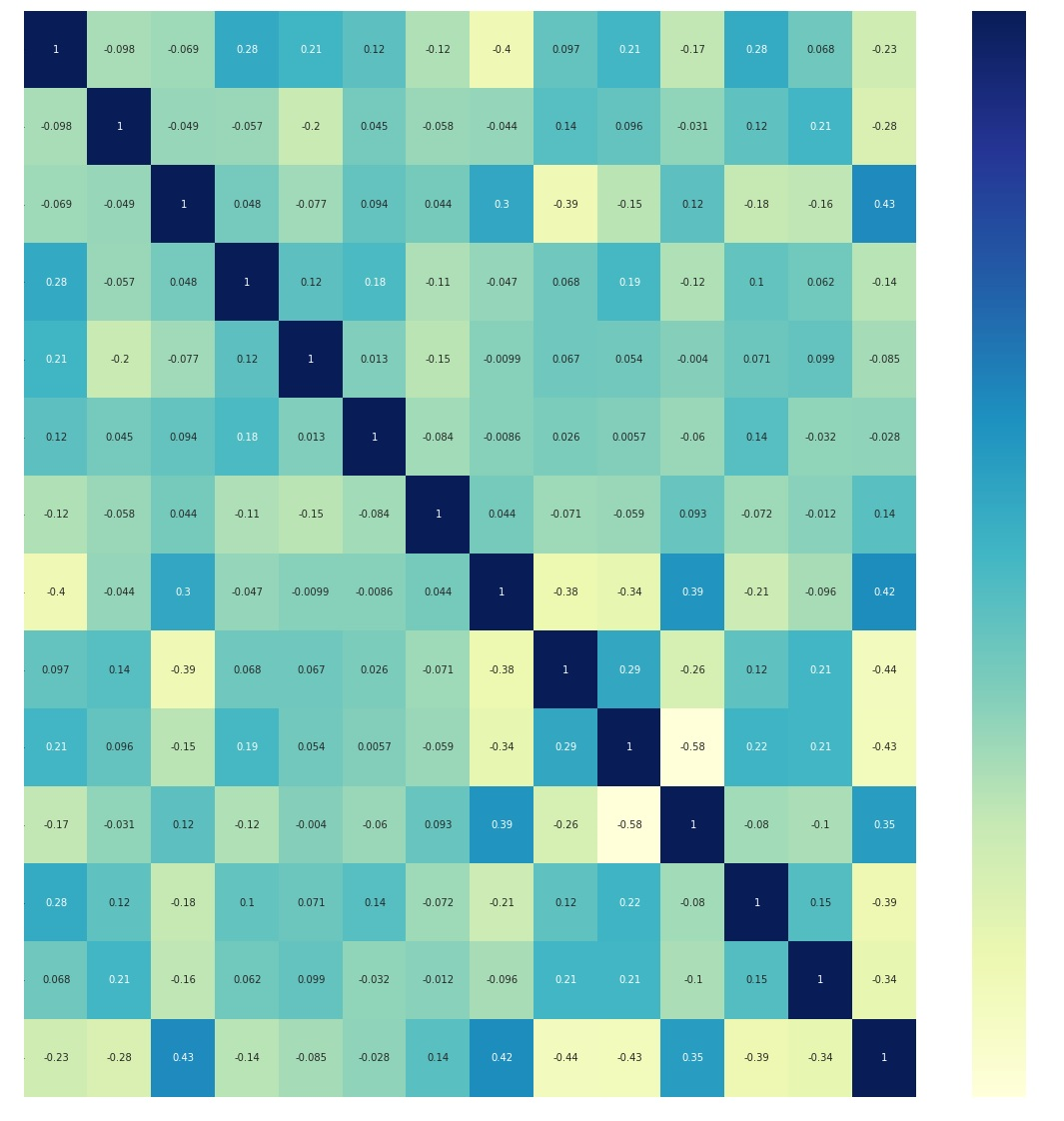
Figure 1. Correlation heatmap of dataset variables.
Based on the correlation heatmap above, the bottom-most row and right-most column depict the correlation of each factor with the target. From the correlation heat map, it is evident that cp, thalach are the most positively correlated with the target, and exang, oldpeak, and ca are the most inversely correlated with the target. To summarize, from the correlation heat map, the five features (cp, thalach, exang, oldpeak, ca) depict the most correlation with the target result.
Feature Selection
Using a chi-squared statistical test, we identified the same 5 features as having the highest correlation with the target variable.
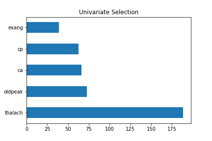
Figure 2. Univariate Selection of five features of the dataset.
The Extra Tree Classifier class in the scikit-learn API was used to estimate the importance of features. The five features displayed were the same as above, but the scores were different from the univariate selection.
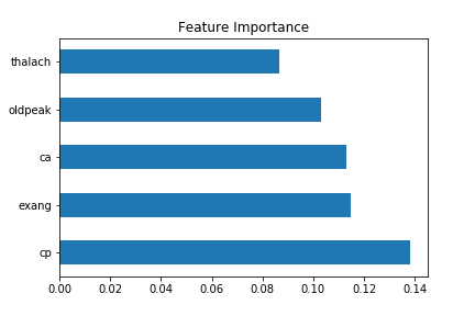
Figure 3. Feature importance.
In order to show the accuracy of the following algorithms to choose the most common risk factors for cardiovascular disease from our dataset, we tried to match it with proven medical research. Our top 5 features from the dataset includes [‘ca’, ‘cp’, ‘exang’, ‘old peak’, ‘thalach’] which essentially breaks down to chest pain, number of major vessels, ST depressions found from an ECG, and a person’s maximum heart rate.
On the other hand, based on research, chest pains, high blood pressure / cholesterol, shortness of breath are among the most common risk factors [2]. We can see that chest pains are a match, as well as shortness of breath and maximum heart rate because they are both correlated to each other. Based on these results, we can see a positive correlation of matches between our dataset and research to show accurate measures.
Normalization
We normalized our raw data in order to convert our data to a common scale and thus have consistency across all four of our models. We also decided to normalize the data because we wanted the training data to not be as sensitive towards the scale of the features. In order to normalize our raw data, we processed it through a Min Max Scaler function from the scikit-learn library. We performed this operation for the machine to train the data easily.
Encoding original values to categorical values

Figure 4. Normalizing age values by categorizing them into five different groups.
Because the original values in ‘age’, ‘trestbps’, ‘chol’, ‘thalach’, ‘oldpeak’ features are not categorical values, we encoded their numerical values into indicator/ categorical values. By doing so, we wanted to see if data manipulation would improve ML training and help us to gain more insight.
Supervised Learning Techniques
Decision Tree
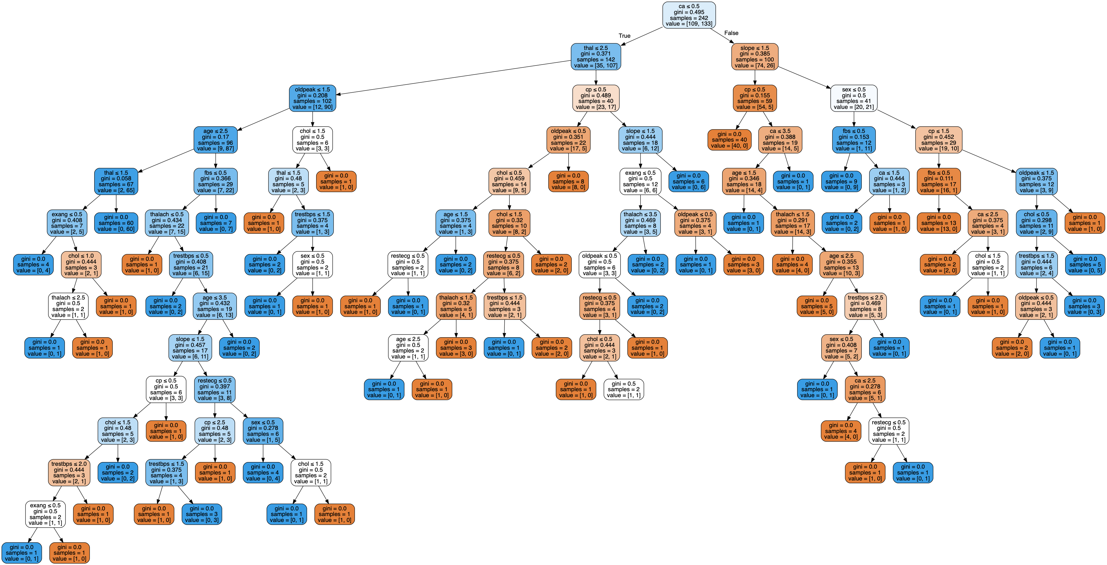
Figure 6. Decision Tree, using Categorized data.
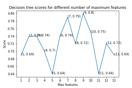
Figure 7. Decision Tree Scores with varying number of maximum features.
Since each node or leaf in the decision tree classifier represents a label / indicator value, it would not make sense to use the original numerical values (non-categorical values) from our raw data. Thus, we only used our processed data where all the numerical values were converted into categorical (indicator) values.
The performance of a decision tree can be increased by pruning. Pruning involves removing the “branches” that are weak in providing classification. Thus, we tried to prune and optimize by changing our decision tree model by changing the number of features used to find the best split in our tree. Our result showed us that having a maximum of 9 features yielded the best accuracy of 80.3%.
Although the accuracy of the decision tree algorithm (80.3%) seems relatively high, from the graph above, we can see that the accuracy fluctuates significantly as the maximum number of features used changes; therefore, it fails to draw a clear pattern or relationship between the maximum number of features and scores. Therefore, it is hard to conclude whether a decision tree classifier is a suitable model for our dataset.
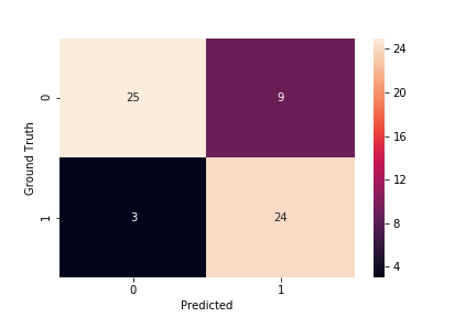
Figure 8. Decision Tree Confusion Matrix
Using the indicator data, the accuracy was 80.3%, specificity was 73.5%, and sensitivity was 88.9%.
Support Vector Machine
Support vector machines are a supervised learning technique where labeled training data is used to generate an optimal hyperplane that separates the two classes and can categorize new testing data. In the case of this study, the SVMs are intended to separate between the two classes of target = 1 and target = 0. Tuning parameters for support vector machines include the regularization parameter, kernel, and gamma. The regularization parameter essentially determines how much you want to avoid misclassifying training examples. The kernel allows the SVM to calculate the separating plane in higher dimensions. Gamma defines how far the influence of a single point reaches, with low values taking into account further points and high values only taking into account the closest points to the hyperplane.
A grid search was conducted to determine the optimal combination of parameters to improve the SVM’s classification accuracy. Based on the grid search, the default values provided in the sklearn library were already the most optimal. The confusion matrices for the optimal SVM parameters using the normalized and indicator data are shown below.
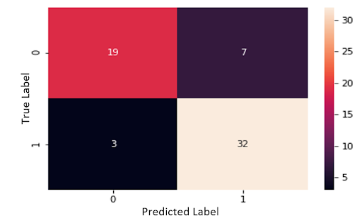
Figure 9. Support Vector Table, Normalized, Categorized
Using the normalized data, the SVM had a total accuracy of 83.6%, a specificity of 73.1%, and a sensitivity of 91.4%. The proportion of false negatives was 4.9%.
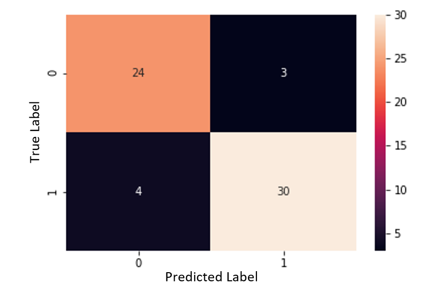
Figure 10. Support Vector Table, Normalized, Non-Categorized
Using the indicator data, the accuracy was 88.5%, specificity was 88.9%, and sensitivity was 88.2%. The proportion of false negatives was 6.6%. With the SVM, it is evident that specificity and overall accuracy increased when training with the indicator data, but sensitivity and the proportion of false negatives suffered very slightly. Because the number of false negatives was so low in general, the slight increase in false negatives is not extremely significant, although it should still be considered when comparing the use of raw and indicator data.
Logistic Regression
Logistic Regression is a supervised classification technique that is used to predict the probability that an input belongs to each class. In this case, we have two target classifications, 0 and 1, which will be our categorical dependent variables.
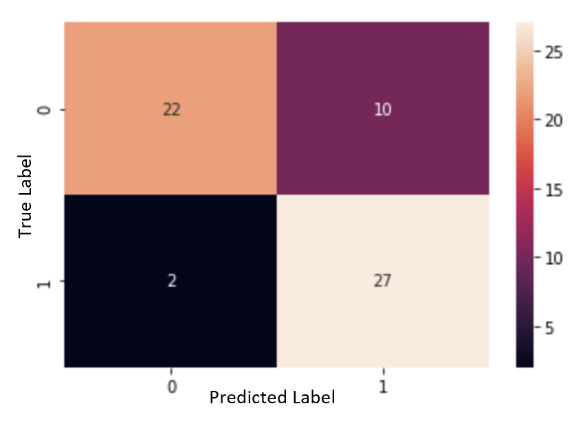
Figure 11. Logistic Regression, Normalized, Non-Categorized
When utilizing the normalized raw data, the logistic regression algorithm had an accuracy of 80.3%, specificity of 68.8%, and sensitivity of 93.1%. The proportion of false negatives was 3.3%.
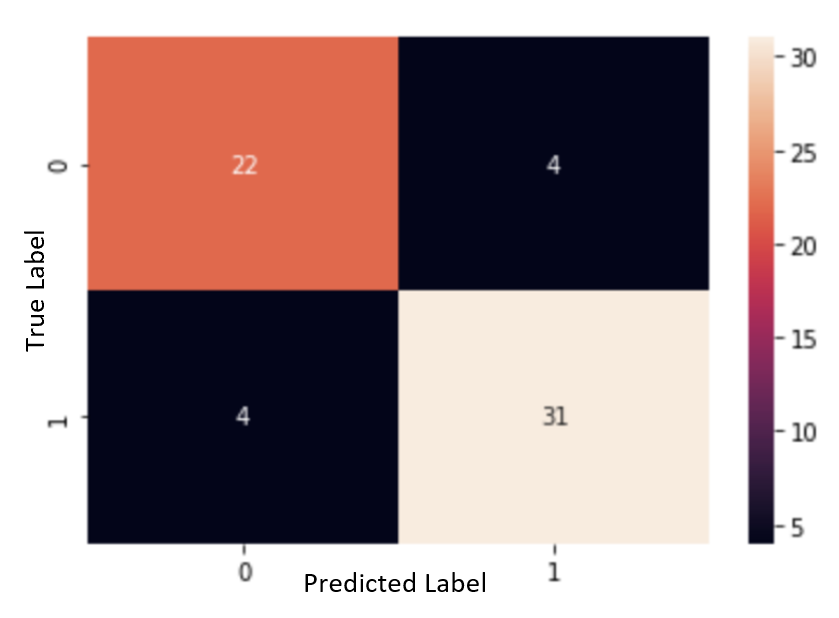
Figure 12. Logistic Regression, Normalized, Categorized
With the indicator data, the accuracy is 86.9%, the specificity is 84.6%, and the sensitivity was 88.5%. The proportion of false negatives was 6.5%.
For Logistic Regression, using the indicator data significantly increased the accuracy, specificity, and proportion of false negatives, while the sensitivity decreased. The increase in the proportion of false negatives was not immense, but it should still be taken into consideration when comparing the normalized data and the indicator data.
The ROC curve helps us to visualize the plotting of the sensitivity and specificity values on a graph. A model that has high discrimination will have a plot that gravitates toward the top left. On the other hand, a model with low discrimination will be closer to the red linear line. The most optimal way to determine if a model has a good discrimination ability is to calculate the area under the ROC curve. This is displayed in the graphs below.
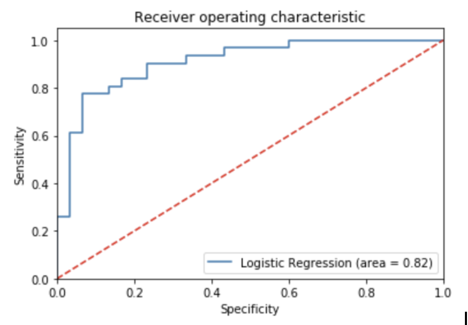
Figure 13. ROC Curve of Logistic Regression, Normalized, Categorized
The ROC curve for the normalized data is displayed above. The area under the curve is 0.82.
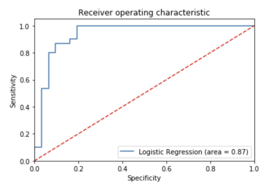
Figure 14. ROC Curve of Logistic Regression, Normalized, Non-Categorized
The ROC curve for the indicator data is displayed above. The area under the curve is 0.87 which is slightly higher than the area for the normalized data model.
Results
In conclusion, the model with the highest performance for heart disease diagnosis is a Support Vector Machine using indicator data with parameters of c = 1, gamma = 1, and kernel = rbf.
Reference
[1] “About Cardiovascular Diseases.” World Health Organization. World Health Organization, September 29, 2011. https://www.who.int/cardiovascular_diseases/about_cvd/en/.
[2] “Coronary Artery Disease.” Mayo Clinic. Mayo Foundation for Medical Education and Research, May 16, 2018. https://www.mayoclinic.org/diseases-conditions/coronary-artery-disease/symptoms-causes/syc-20350613?fbclid=IwAR1vuj1Re0t5CCxKahfVQZn1udRXqawquDE4AcCi-xB-WGJCG5BsKgF2ArU.
[3] “Machine Learning Can Predict Heart Attack or Death More Accurately Than Humans.” AJMC. Accessed November 18, 2019. https://www.ajmc.com/newsroom/machine-learning-can-predict-heart-attack-or-death-more-accurately-than-humans.
[4] “Patient Portal.” Alaska Heart & Vascular Institute. Accessed November 18, 2019. https://www.alaskaheart.com/the-importance-of-the-early-detection-of-cardiovascular-disease/.